Genomic data analysis with large matrices in R
Florian Privé
October 21, 2017
For multiple genomic data, most of the information can be stored as matrices. The most striking example is with SNP data, which can be stored as matrices with thousands to hundreds of thousands of rows (samples) with hundreds of thousands to dozens of millions of columns (SNPs) (Bycroft et al. 2018). This results in datasets of GygaBytes to TeraBytes of data.
Other fields in genomics, such as proteomics or expression data, use data stored as matrices potentially of size larger than available memory.
To address large data size in R, we can use memory-mapping for accessing large matrices stored on disk instead of in RAM. This has existed in R for several years thanks to package {bigmemory} (Kane, Emerson, and Weston 2013).
More recently, two packages that use the same principle as bigmemory have been developed: {bigstatsr} and {bigsnpr} (Privé et al. 2018). Package {bigstatsr} implements many statistical tools for several types of Filebacked Big Matrices (FBMs), making it usable for any type of genomic data that can be encoded as a matrix. The statistical tools in {bigstatsr} include implementation of multivariate sparse linear models, truncated Principal Component Analysis (PCA), matrix operations, and numerical summaries. Package {bigsnpr} implements algorithms that are specific to the analysis of SNP arrays, making use of already implemented features in package {bigstatsr}.
In this small tutorial, we see the potential benefits of using memory-mapping instead of standard R matrices in memory, by using {bigstatsr} and {bigsnpr}.
Examples
Example of expression data
Let’s use the NCBI GEO archive to get some example expression data (Barrett et al. 2012).
# http://bioconductor.org/packages/release/bioc/html/GEOquery.html
suppressMessages(library(GEOquery))

# All data
gds <- getGEO("GDS3929")
## File stored at:## /tmp/RtmpOTdb2V/GDS3929.soft.gzstr(gds, max.level = 2)## Formal class 'GDS' [package "GEOquery"] with 3 slots
## ..@ gpl :Formal class 'GPL' [package "GEOquery"] with 2 slots
## ..@ dataTable:Formal class 'GEODataTable' [package "GEOquery"] with 2 slots
## ..@ header :List of 23format(object.size(gds), units = "MB")## [1] "37.1 Mb"df <- gds@dataTable@table
format(object.size(df), units = "MB")## [1] "37 Mb"# Part of the data that can be encoded as a matrix
mat <- t(df[-(1:2)])
dim(mat)## [1] 183 24526format(object.size(mat), units = "MB")## [1] "35.6 Mb"In this data, 96% of the information can be encoded as a matrix. For larger data, this could increase to more than 99%. Let us store this as a Filebacked Big Matrix (FBM).
# devtools::install_github("privefl/bigstatsr")
library(bigstatsr)
fbm <- as_FBM(mat)
# Same data?
all.equal(fbm[], mat, check.attributes = FALSE)
## [1] TRUE# Size in memory
format(object.size(fbm), units = "MB")## [1] "0 Mb"# File where the data is backed
fbm$backingfile## [1] "C:\\Users\\Florian\\AppData\\Local\\Temp\\Rtmps7eEQV\\file1bbc9c85c43.bk"So, now the matrix is stored on disk and basically takes no memory.
For omic data, computing PCA (or SVD) is sometimes useful to assess the structure in the data. Let’s do this.
system.time(
  svd <- svd(scale(mat), nu = 10, nv = 10)
)
## user system elapsed
## 2.265 0.042 2.316plot(svd$u)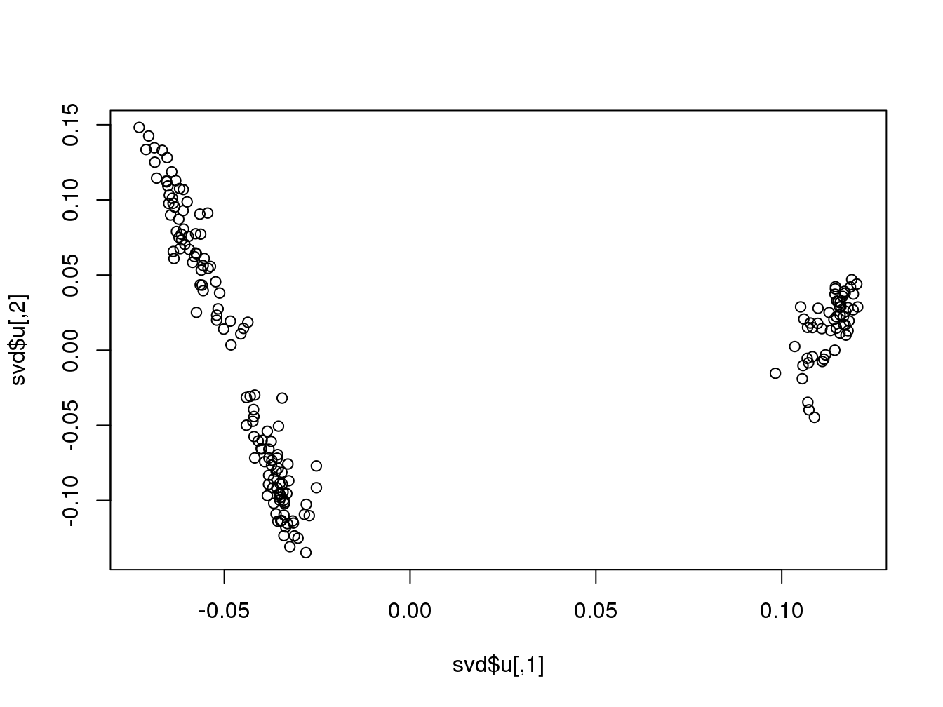
system.time(
  svd2 <- big_SVD(fbm, big_scale(), k = 10)
) # see big_randomSVD() for very large data
## user system elapsed
## 0.74 0.12 0.88plot(svd2)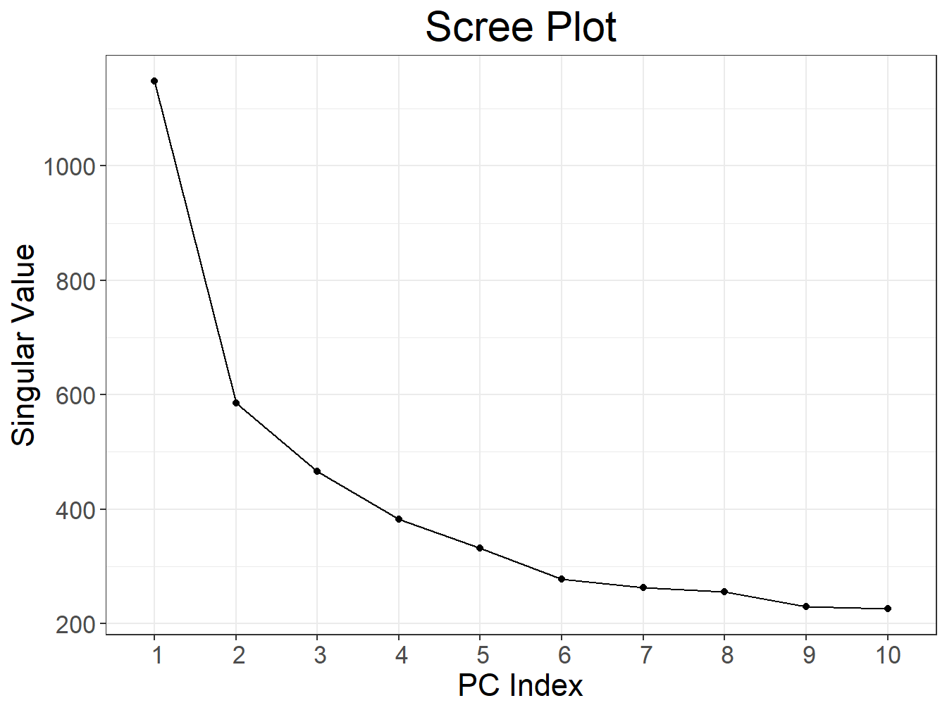
plot(svd2, type = "scores")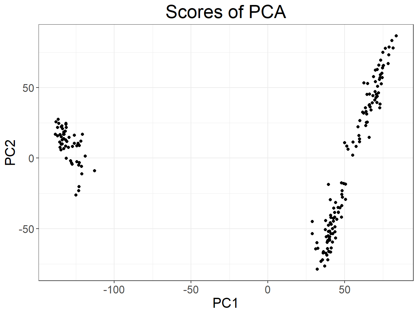
The goal of memory-mapping is to not have all the data in memory. This force programmers to think more before implementing algorithms. This can lead to implementations that can be much faster than current R implementations. Moreover, data stored on disk is shared between processes so that parallelism in algorithms can be implemented more easily and efficiently, for example removing the need to copy the data to each core.
Example of SNP data
Let’s use some data from Gad Abraham’s GitHub repository that have been filtered and quality-controled.
tmpfile <- tempfile()
base <- paste0(
  "https://github.com/gabraham/flashpca/raw/master/HapMap3/",
  "1kg.ref.phase1_release_v3.20101123_thinned_autosomal_overlap")
exts <- c(".bed", ".bim", ".fam")
purrr::walk2(paste0(base, exts), paste0(tmpfile, exts), ~download.file(.x, .y))
First, we have to transform these data in PLINK format to an FBM. In package {bigsnpr}, function snp_readBed() is provided to do just that. It is implemented with Rcpp, which makes it very fast. Package {Rcpp} makes easy to use C++ code in R and with R objects.
# https://github.com/privefl/bigsnpr
library(bigsnpr)
rdsfile <- snp_readBed(paste0(tmpfile, ".bed"))
## Warning in snp_readBed(paste0(tmpfile, ".bed")): EOF of bedfile has not been reached.bigsnp <- snp_attach(rdsfile)
(G <- bigsnp$genotypes)## A Filebacked Big Matrix of type 'code 256' with 1092 rows and 14079 columns.object.size(G)## 688 bytesG[which(is.na(G[]))] <- 0 # quick and dirty imputation
G.matrix <- G[]
format(object.size(G.matrix), units = "MB")## [1] "117.3 Mb"For large SNP data, this format can save us a lot of memory.
system.time(
  svd <- svd(scale(G.matrix), nu = 10, nv = 10)
)
## user system elapsed
## 9.154 0.741 9.895plot(svd$u)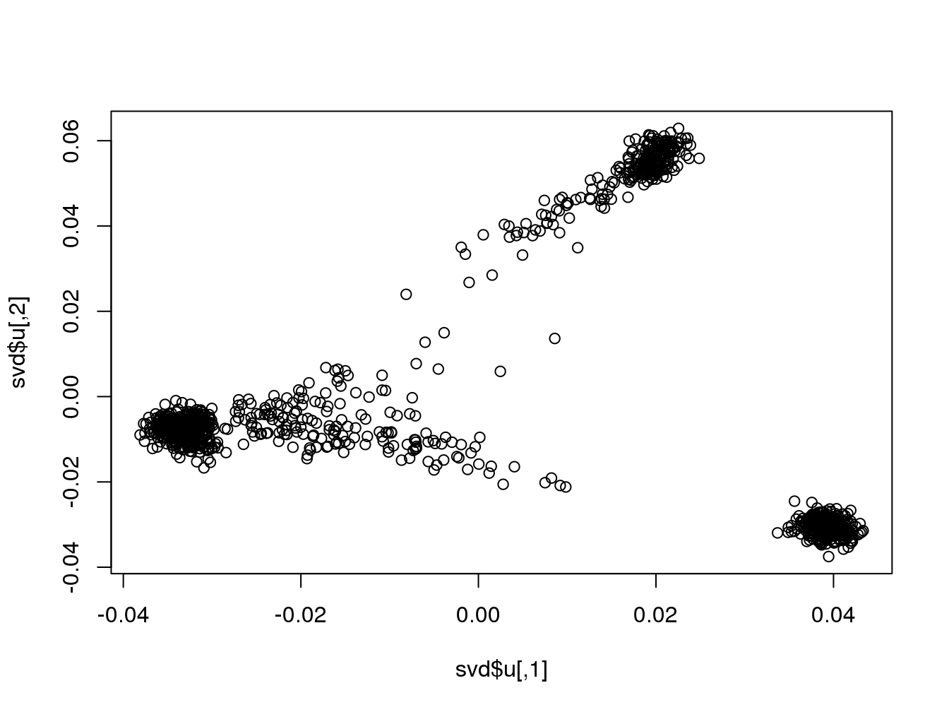
system.time(
  svd2 <- big_SVD(G, big_scale(), k = 10)
)
## (2)## user system elapsed
## 0.941 0.045 0.986plot(svd2)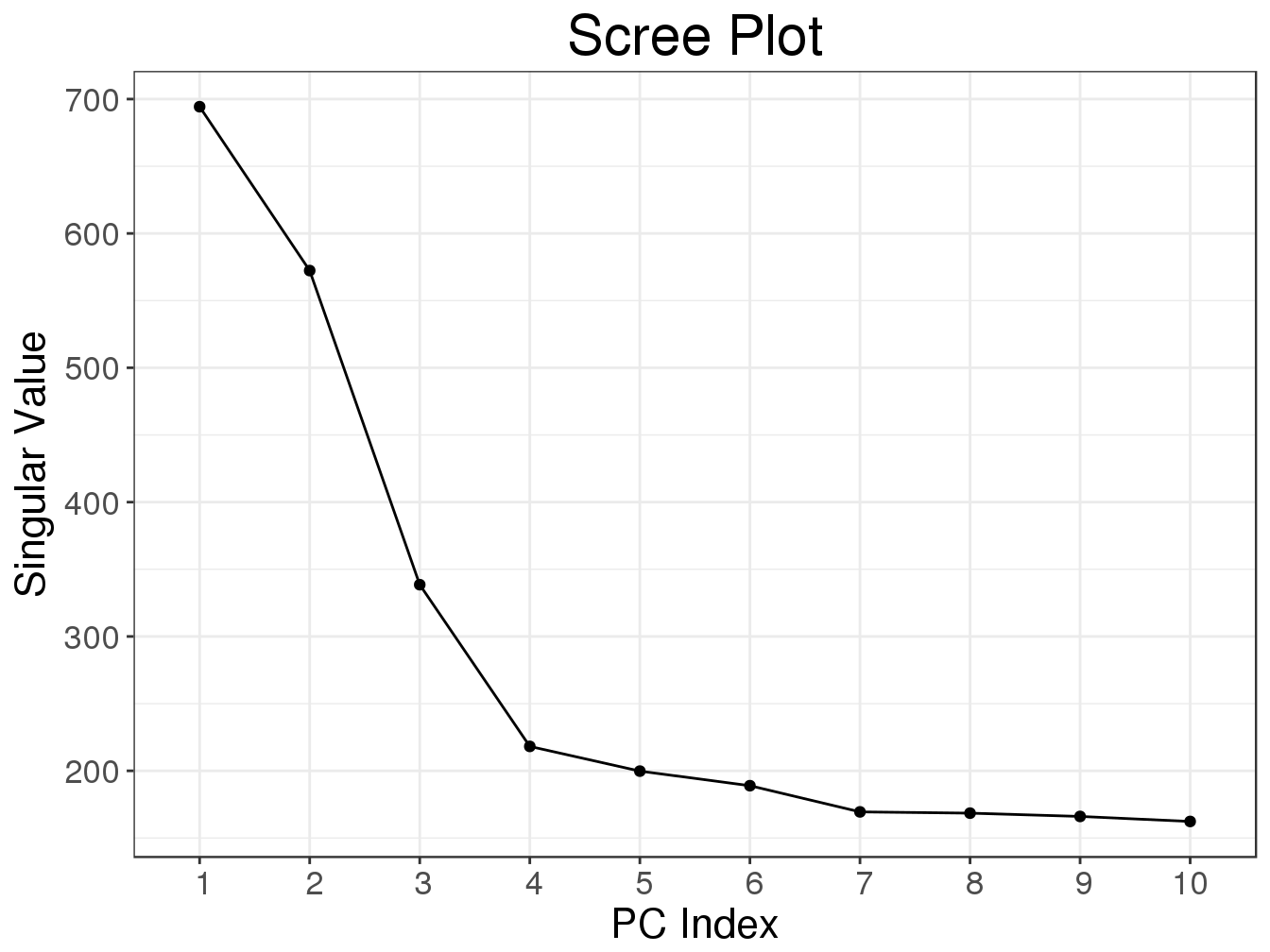
plot(svd2, type = "scores")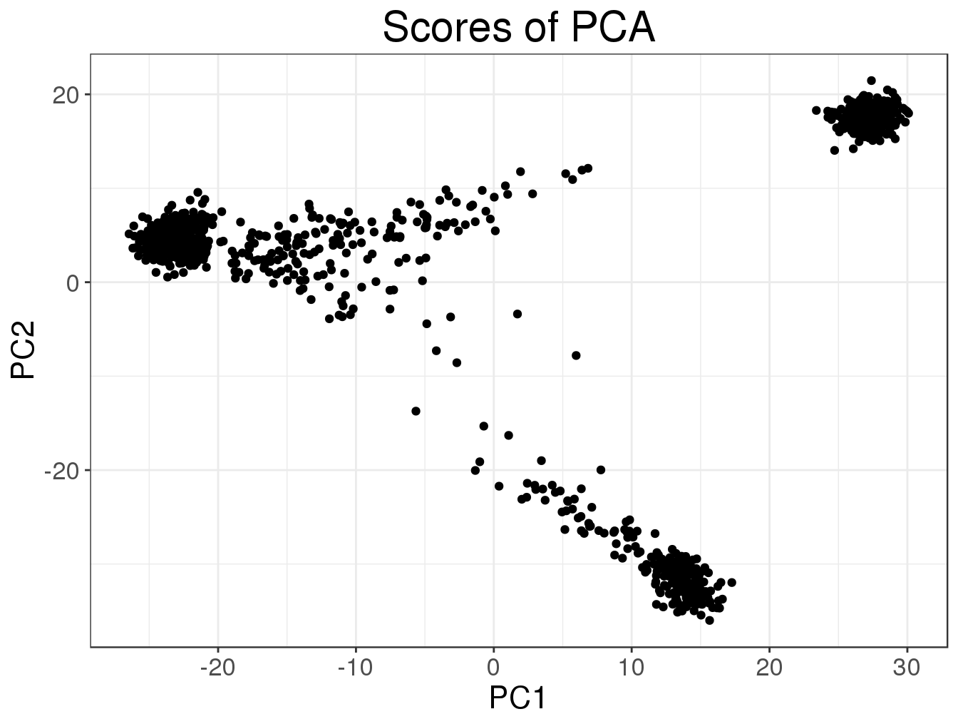
Learn more
You can find vignettes and documentation of packages {bigstatsr} and {bigsnpr} in their GitHub repositories. In order to find more details about memory-mapping and these packages, please refer to the corresponding paper (Privé et al. 2018).
For instance, you will see that when using memory-mapping, it is possible to make a parallelized algorithm for computing partial Singular Value Decomposition that is lightning fast, using an already implemented algorithm in another R package.
You’ll also see that it is possible to make a Genome-Wide Association Study (GWAS) on 500,000 individuals genotyped on more than 1,000,000 SNPs, thus analyzing more than 100 GB of compressed data on a single desktop computer.
References
Barrett, Tanya, Stephen E Wilhite, Pierre Ledoux, Carlos Evangelista, Irene F Kim, Maxim Tomashevsky, Kimberly A Marshall, et al. 2012. “NCBI Geo: Archive for Functional Genomics Data Sets—update.” Nucleic Acids Research 41 (D1). Oxford University Press: D991–D995.
Bycroft, Clare, Colin Freeman, Desislava Petkova, Gavin Band, Lloyd T Elliott, Kevin Sharp, Allan Motyer, et al. 2018. “The Uk Biobank Resource with Deep Phenotyping and Genomic Data.” Nature 562 (7726). Nature Publishing Group: 203.
Kane, Michael J, John W Emerson, and Stephen Weston. 2013. “Scalable Strategies for Computing with Massive Data.” Journal of Statistical Software 55 (14): 1–19. doi:10.18637/jss.v055.i14.
Privé, Florian, Hugues Aschard, Andrey Ziyatdinov, and Michael G B Blum. 2018. “Efficient Analysis of Large-Scale Genome-Wide Data with Two R Packages: Bigstatsr and Bigsnpr.” Bioinformatics 34 (16): 2781–7. doi:10.1093/bioinformatics/bty185.