Doing all your analysis in R

A biological analysis is sometimes more appropriately called a pipeline. This is because it generally consists of many steps, using many different software and data formats. Yet, these analysis pipelines are becoming very complex and usually makes use of bash/perl scripts. For people like me who don’t really know that much bash or perl, it can be really hard to understand those scripts.

What is important in these pipelines? To list what comes to my mind:

use the command line
manipulate files
use regular expressions
visualize results
report results

I think we could do each of these operations in R. And I think we should.

The main reason would be to put all your analysis in a single notebook where you have all your code, results and possibly some writing. Using notebooks is good practice and makes it possible to have a fully reproducible analysis, which will become a standard in years to come. Another reason is simply that it is easier!

In this tutorial, I show an example of a moderately complex analysis of the HapMap3 data (phase III), all in R.

Example with HapMap3

Get the data

Do not just give a link to the data, use an R command to download the data directly. Mouse clicks prevent reproducibility.

# Get the URL of the data
site <- "https://ftp.ncbi.nlm.nih.gov/hapmap/genotypes/2009-01_phaseIII/plink_format/"
name <- "hapmap3_r2_b36_fwd.qc.poly"
ext <- ".tar.bz2"

# Download the file 
download.file(paste0(site, name, ext), tmp <- tempfile(fileext = ext))
# Uncompress the downloaded file in directory data/
untar(tmp, exdir = "data")

Use PLINK to combine datasets

PLINK is a very efficient command-line software very useful for preprocessing of genome-wide data (Chang et al. 2015; S. Purcell et al. 2007).

# devtools::install_github("privefl/bigsnpr")
plink <- bigsnpr::download_plink()

files <- rev(list.files("data/hapmap3_pop", full.names = TRUE))
write(files, tmp <- tempfile(), ncolumns = 2)
library(glue)
system(glue("{plink} --merge-list {tmp} --out data/hapmap3"))

Use PLINK for quality control

system(glue(
  "{plink} --bfile data/hapmap3",
  " --maf 0.05",
  " --geno 0.05", 
  " --hwe 1e-10", 
  " --autosome",
  " --make-bed",
  " --out data/hapmap3_qc"
))

There exists much more quality control steps but it is not the objective of this tutorial. For details, please refer to (Anderson et al. 2010).

Get a pruned dataset

First, we need to remove long-range LD regions and use pruning.

# Write long-range LD regions in a file
bigsnpr:::write.table2(bigsnpr::LD.wiki34, tmp <- tempfile())
# Get pruned SNPs
system(glue("{plink} --bfile data/hapmap3_qc",
            " --exclude {tmp} --range",
            " --indep-pairwise 50 5 0.2",
            " --out {tmp}"))

Compute Principal Components

# Compute first PCs based on pruned SNPs using PLINK
system(glue("{plink} --bfile data/hapmap3_qc",
            " --extract {tmp}.prune.in",
            " --pca",
            " --out {tmp}"))

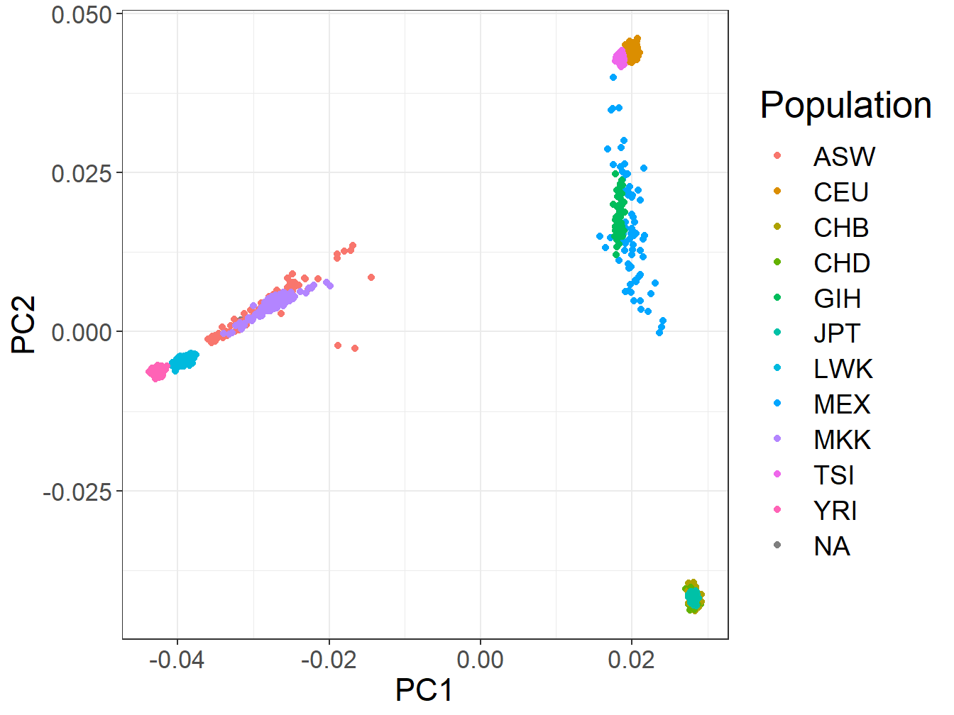
# Get result and plot it (data.table is faster for reading/writing files)
readLines(glue("{tmp}.eigenvec"), n = 3)

## [1] "1328 NA06984 0.020195 0.044255 -0.0100406 -0.0168748 0.0226282 0.00355131 -0.000642671 -0.000914571 0.00227462 -0.00378351 -0.0061861 4.06576e-05 -0.00356761 2.57855e-05 0.00430737 0.00157184 0.000507544 -0.000671943 0.00237496 0.0055083"
## [2] "1328 NA06989 0.0196734 0.0433813 -0.00835398 -0.0150484 0.0216197 -0.00347001 0.000290989 0.00110012 -0.000879973 0.00799929 0.000625262 0.00226367 -0.00617662 0.00371815 0.0019478 0.0024499 -0.000891975 0.00197824 0.00205231 -0.00154855"
## [3] "1330 NA12335 0.0198508 0.0445815 -0.0105505 -0.0187938 0.0220378 -0.000335578 0.0035803 -0.0031238 0.00734259 0.00405858 -0.00266854 -0.00517518 0.00611168 -0.00197511 0.0116496 0.00503205 0.00181431 -0.00481878 0.00798023 0.000464057"

evec <- data.table::fread(glue("{tmp}.eigenvec"), data.table = FALSE)

# Get population info
txt <- "relationships_w_pops_121708.txt"
download.file(paste0(site, txt), paste0("data/", txt))
info <- data.table::fread(paste0("data/", txt), data.table = FALSE)
fam <- data.table::fread("data/hapmap3_qc.fam", data.table = FALSE)
fam <- dplyr::left_join(fam, info, by = c("V1" = "FID", "V2" = "IID"))


library(ggplot2)
ggplot(evec) + 
  bigstatsr::theme_bigstatsr() +
  geom_point(aes(V3, V4, color = fam$population)) +
  labs(x = "PC1", y = "PC2", color = "Population")

Discussion

It would be easy to make functions that implements whole procedures in R thanks to system calls and package glue. This could make pipelines more understandable and fully reproducible.

References

Anderson, Carl A, Fredrik H Pettersson, Geraldine M Clarke, Lon R Cardon, Andrew P Morris, and Krina T Zondervan. 2010. “Data Quality Control in Genetic Case-Control Association Studies.” Nature Protocols 5 (9). Europe PMC Funders: 1564.

Chang, Christopher C, Carson C Chow, Laurent CAM Tellier, Shashaank Vattikuti, Shaun M Purcell, and James J Lee. 2015. “Second-Generation Plink: Rising to the Challenge of Larger and Richer Datasets.” Gigascience 4 (1). BioMed Central: 7.

Purcell, Shaun, Benjamin Neale, Kathe Todd-Brown, Lori Thomas, Manuel AR Ferreira, David Bender, Julian Maller, et al. 2007. “PLINK: A Tool Set for Whole-Genome Association and Population-Based Linkage Analyses.” The American Journal of Human Genetics 81 (3). Elsevier: 559–75.